Introduction
ReboundTools is an R package that provides
functions to analyze energy rebound,
the unanticipated reduction of the benefits of energy efficiency due to
behavior change and economy-wide effects. Many functions (described in
the ReboundTools vignette) perform analysis calculations to
move from known parameters to rebound estimates. Graphing functions
create rebound path graphs in energy, expenditure, and consumption
spaces. Other graphing functions create sensitivity graphs. The
functions in this package were used for the analyses and graphs in the
paper **********.
Rebound path graphs
Rebound graphs can be created with the path_graphs()
function. Three types of rebound graphs are available:
- Energy paths,
- Expenditure paths, and
- Consumption paths.
The graph_type argument to path_graphs()
controls which type of path graph is returned (one of “Energy”,
“Expenditure”, or “Consumption”). By default, all three graph types are
returned. The cases argument determines which cases are
plotted. By default, all cases are returned.
Energy path graph
An energy path graph shows the energy effects of the energy efficiency upgrade, with direct energy consumption on the horizontal axis and indirect energy consumption on the vertical axis. Diagonal lines with negative slope indicate lines of constant energy consumption. The thicker lines show 0 % rebound (lower left) and 100 % rebound (upper right). Thinner lines show rebound after each effect in order from the 0 % line to the 100 % line: emplacement, substitution, income, and macro. The following example illustrates an energy path graph.
load_eeu_data() %>%
  rebound_analysis() %>%
  path_graphs(cases = "Car", graph_types = "Energy") +
  ggplot2::theme_classic()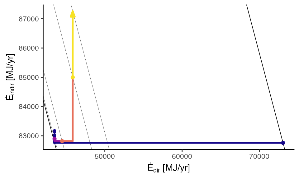
Expenditure path graph
The expenditure path graph shows expenditures for rebound effects. Direct expenditures for the energy service (including substitution and income takebacks) are shown in the horizontal axis; capital expenditures, maintenance and disposal expenditures, substitution effect savings, and income effect expenditures are shown in the vertical axis. Diagonal lines with negative slope indicate lines of constant expenditure. The lower-left line indicates expected expenditure options before capital expenditure changes, maintenance expenditure changes, or behavior changes. Note that the beginning (dot) and end (arrow) of the expenditure path both lie on the same expenditure line, indicating that all freed cash (after the emplacement and substitution effects) is re-spent in the income effect.
load_eeu_data() %>%
  rebound_analysis() %>%
path_graphs(cases = "Car", graph_types = "Expenditure") +
  ggplot2::theme_classic()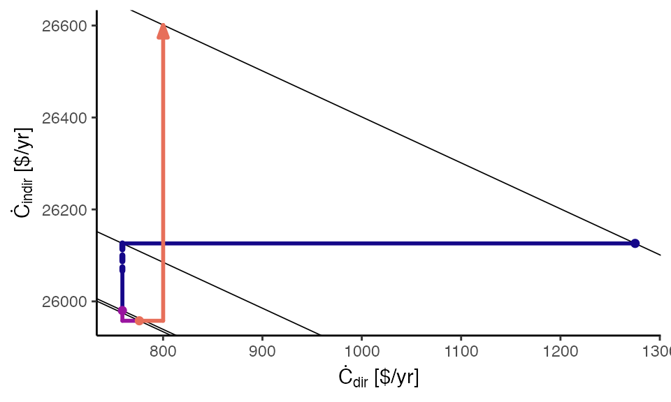
Consumption path graph
The consumption path graph shows details of the substitution and income effects, with normalized energy service consumption on the horizontal axis and normalized expenditures on other goods on the vertical axis. Diagonal grid lines with negative slope indicate constant expenditure sum of the energy service (horizontal axis) and other goods (vertical axis). Negative-sloping lines show the tradeoff between consumption of the energy service (horizontal axis) and consumption of other goods (vertical axis). The swooping, concave-upward grid lines indicate lines of constant utility: indifference curves.
load_eeu_data() %>%
  rebound_analysis() %>%
  path_graphs(cases = "Car", graph_types = "Consumption") +
  ggplot2::xlim(0.995, 1.06) +
  ggplot2::ylim(0.995, 1.04) +
  ggplot2::theme_classic()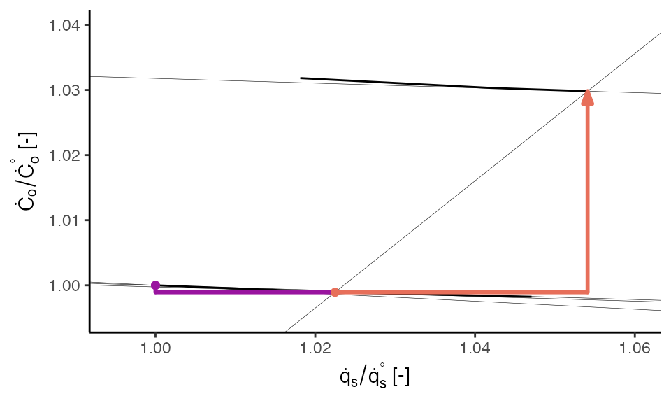
Arguments to path_graphs()
In addition to the graph_types and cases
arguments, the following arguments adjust the composition and appearance
of graphs:
-
indexed, -
graph_types, -
grid_types, and graph_params.
indexed
Setting indexed = TRUE normalizes the rebound data to
conditions before emplacement of the energy efficient device, such that
the starting point is always (1, 1).
load_eeu_data() %>%
  rebound_analysis() %>%
  path_graphs(indexed = TRUE, cases = "Car", graph_types = "Energy") +
  ggplot2::theme_classic()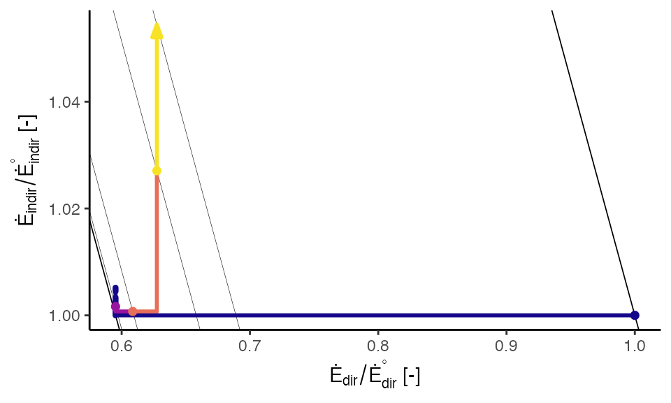
As discussed above, the cases argument tells which
Cases should be plotted. All cases are plotted by default,
although the result is rarely pleasing.
load_eeu_data() %>%
  rebound_analysis() %>%
  path_graphs(cases = c("Car", "Lamp"),
                   graph_types = "Energy") +
  ggplot2::theme_classic()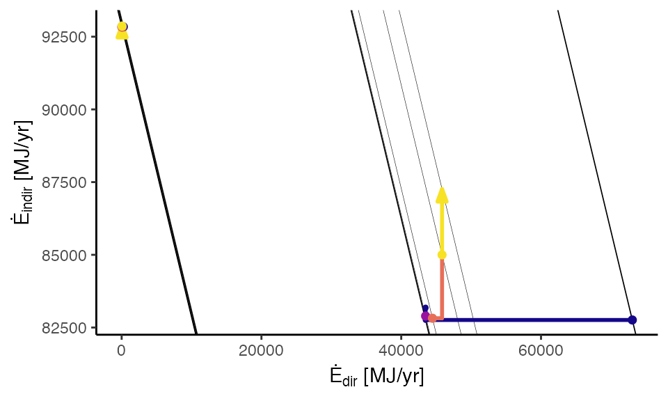
When the cases are overlapping or very different (as above), faceting and indexing may improve the appearance of the graph.
load_eeu_data() %>%
  rebound_analysis() %>%
  path_graphs(indexed = TRUE,
                   graph_types = ReboundTools::graph_types$energy) +
    ggplot2::facet_wrap(facets = ReboundTools::eeu_base_params$case) +
  ggplot2::theme_classic()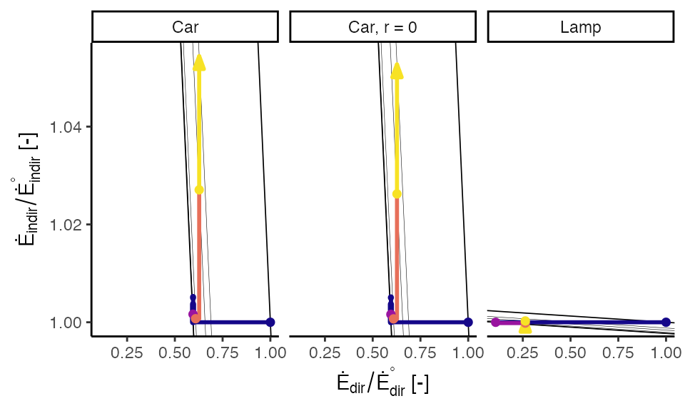
graph_types
The graph_types argument tells which type of graph
should be created. The default ReboundTools::graph_types
returns all three graph types. Again, faceting and indexing may be
beneficial.
load_eeu_data() %>%
  rebound_analysis() %>%
  path_graphs(indexed = TRUE, cases = "Car") +
  ggplot2::facet_wrap(facets = ReboundTools::graph_df_colnames$graph_type_col) +
  ggplot2::xlim(0.5, 1.2) +
  ggplot2::ylim(0.99, 1.08) +
  ggplot2::theme_classic()
#> Warning: Removed 188 rows containing missing values or values outside the scale range
#> (`geom_line()`).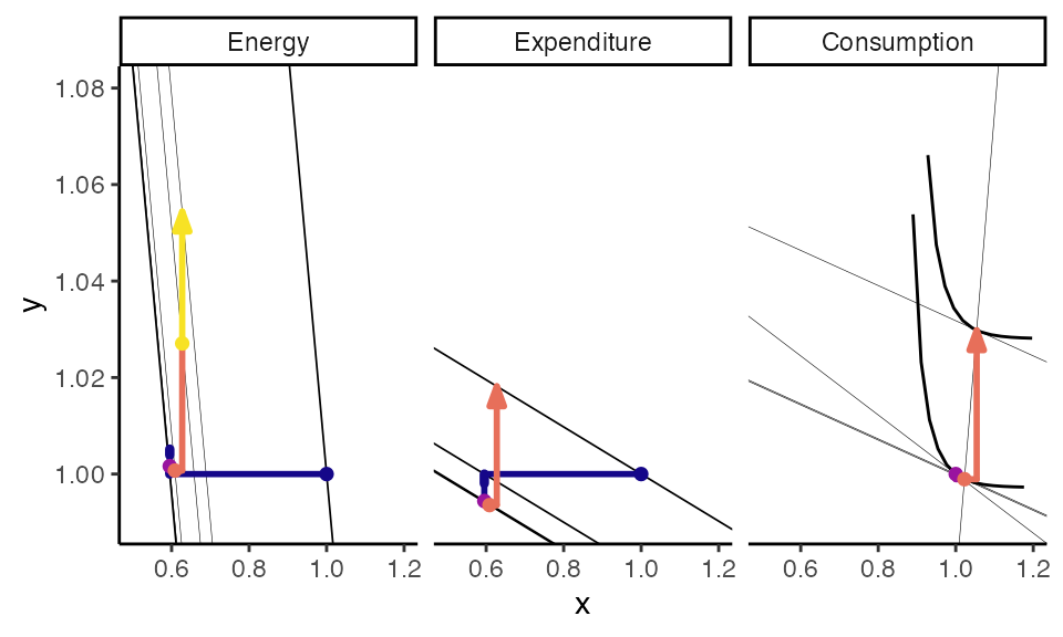
Note that the path_graphs() function applies labels to
the x and y axes whenever the labels are unambiguous. However, when
multiple path graphs are included in the same figure, the x and y axis
labels are unclear. The user can apply labels appropriate to their
situation.
load_eeu_data() %>%
  rebound_analysis() %>%
  path_graphs(indexed = TRUE, cases = "Car") +
  ggplot2::facet_wrap(facets = ReboundTools::graph_df_colnames$graph_type_col) +
  ggplot2::xlim(0.5, 1.2) +
  ggplot2::ylim(0.99, 1.08) +
  ggplot2::xlab("my x label") +
  ggplot2::ylab("my y label") +
  ggplot2::theme_classic()
#> Warning: Removed 188 rows containing missing values or values outside the scale range
#> (`geom_line()`).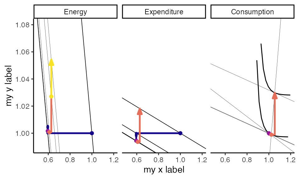
load_eeu_data() %>%
  rebound_analysis() %>%
  path_graphs(indexed = TRUE) +
  ggplot2::facet_grid(rows = vars(Case),
                      cols = vars(graph_type),
                      scales = "free") +
  ggplot2::xlim(0.5, 1.2) +
  ggplot2::ylim(0.99, 1.08) +
  ggplot2::theme_classic()
#> Warning: Removed 335 rows containing missing values or values outside the scale range
#> (`geom_line()`).
#> Warning: Removed 12 rows containing missing values or values outside the scale range
#> (`geom_segment()`).
#> Warning: Removed 1 row containing missing values or values outside the scale range
#> (`geom_segment()`).
#> Removed 1 row containing missing values or values outside the scale range
#> (`geom_segment()`).
#> Removed 1 row containing missing values or values outside the scale range
#> (`geom_segment()`).
#> Warning: Removed 3 rows containing missing values or values outside the scale range
#> (`geom_segment()`).
#> Warning: Removed 6 rows containing missing values or values outside the scale range
#> (`geom_point()`).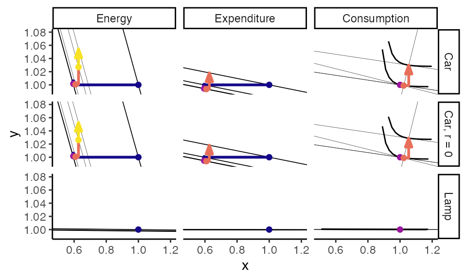
grid_types
The grid_types argument tells which grids to include on
the rebound graphs. By default, grids are provided for all graph types.
In the example below, grids are provided only for the energy and
expenditure path graphs.
load_eeu_data() %>%
  rebound_analysis() %>%
  path_graphs(indexed = TRUE, grid_types = c("Energy", "Expenditure")) +
  ggplot2::facet_grid(rows = vars(Case),
                      cols = vars(graph_type),
                      scales = "free") +
  ggplot2::xlim(0.5, 1.2) +
  ggplot2::ylim(0.99, 1.08) +
  ggplot2::theme_classic()
#> Warning: Removed 12 rows containing missing values or values outside the scale range
#> (`geom_segment()`).
#> Warning: Removed 1 row containing missing values or values outside the scale range
#> (`geom_segment()`).
#> Removed 1 row containing missing values or values outside the scale range
#> (`geom_segment()`).
#> Removed 1 row containing missing values or values outside the scale range
#> (`geom_segment()`).
#> Warning: Removed 3 rows containing missing values or values outside the scale range
#> (`geom_segment()`).
#> Warning: Removed 6 rows containing missing values or values outside the scale range
#> (`geom_point()`).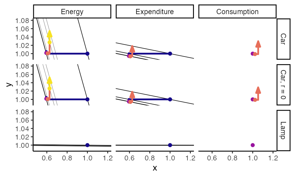
graph_params
While indexed controls how the data are
quantified and graph_types and grid_types
control what data are shown, graph_params controls
the appearance of rebound graphs. graph_params
should be a named list. The default graph_params list is
path_graph_params.
ReboundTools::path_graph_params
#> $which_points
#> # A tibble: 5 × 2
#>   point_name start_point
#>   <chr>      <lgl>
#> 1 orig       TRUE
#> 2 star       TRUE
#> 3 hat        TRUE
#> 4 bar        TRUE
#> 5 tilde      FALSE
#>
#> $last_point
#> [1] FALSE
#>
#> $point_shape
#> [1] 19
#>
#> $point_size
#> [1] 1
#>
#> $point_stroke
#> [1] 1
#>
#> $which_arrows
#> # A tibble: 9 × 2
#>   line_name end_arrow
#>   <chr>     <lgl>
#> 1 dempl     FALSE
#> 2 emb       FALSE
#> 3 cap       FALSE
#> 4 OMd       FALSE
#> 5 isub      FALSE
#> 6 dsub      FALSE
#> 7 dinc      FALSE
#> 8 iinc      FALSE
#> 9 macro     FALSE
#>
#> $last_arrow
#> [1] TRUE
#>
#> $arrow_style
#> $angle
#> [1] 20
#>
#> $length
#> [1] 0.1inches
#>
#> $ends
#> [1] 2
#>
#> $type
#> [1] 2
#>
#> attr(,"class")
#> [1] "arrow"
#>
#> $show_indifference_curves
#> [1] TRUE
#>
#> $dempl_colour
#> [1] "#150789FF"
#>
#> $emb_colour
#> [1] "#150789FF"
#>
#> $cap_colour
#> [1] "#150789FF"
#>
#> $omd_colour
#> [1] "#150789FF"
#>
#> $empl_colour
#> [1] "#150789FF"
#>
#> $isub_colour
#> [1] "#99149FFF"
#>
#> $dsub_colour
#> [1] "#99149FFF"
#>
#> $sub_colour
#> [1] "#99149FFF"
#>
#> $dinc_colour
#> [1] "#E76F5AFF"
#>
#> $iinc_colour
#> [1] "#E76F5AFF"
#>
#> $inc_colour
#> [1] "#E76F5AFF"
#>
#> $micro_colour
#> [1] "#F7E225FF"
#>
#> $macro_colour
#> [1] "#F7E225FF"
#>
#> $dir_colour
#> [1] "black"
#>
#> $indir_colour
#> [1] "black"
#>
#> $tot_colour
#> [1] "black"
#>
#> $dempl_linewidth
#> [1] 1
#>
#> $emb_linewidth
#> [1] 1.5
#>
#> $cap_linewidth
#> [1] 1.5
#>
#> $omd_linewidth
#> [1] 1
#>
#> $empl_linewidth
#> [1] 1
#>
#> $isub_linewidth
#> [1] 1
#>
#> $dsub_linewidth
#> [1] 1
#>
#> $sub_linewidth
#> [1] 1
#>
#> $dinc_linewidth
#> [1] 1
#>
#> $iinc_linewidth
#> [1] 1
#>
#> $inc_linewidth
#> [1] 1
#>
#> $micro_linewidth
#> [1] 1
#>
#> $macro_linewidth
#> [1] 1
#>
#> $dir_linewidth
#> [1] 1
#>
#> $indir_linewidth
#> [1] 1
#>
#> $tot_linewidth
#> [1] 2
#>
#> $dempl_linetype
#> [1] "solid"
#>
#> $emb_linetype
#> [1] "11"
#>
#> $cap_linetype
#> [1] "11"
#>
#> $omd_linetype
#> [1] "solid"
#>
#> $empl_linetype
#> [1] "solid"
#>
#> $dsub_linetype
#> [1] "solid"
#>
#> $isub_linetype
#> [1] "solid"
#>
#> $sub_linetype
#> [1] "solid"
#>
#> $dinc_linetype
#> [1] "solid"
#>
#> $iinc_linetype
#> [1] "solid"
#>
#> $sinc_linetype
#> [1] "solid"
#>
#> $micro_linetype
#> [1] "solid"
#>
#> $macro_linetype
#> [1] "solid"
#>
#> $dir_linetype
#> [1] "solid"
#>
#> $indir_linetype
#> [1] "solid"
#>
#> $tot_linetype
#> [1] "solid"
#>
#> $lineend
#> [1] "round"
#>
#> $linejoin
#> [1] "round"
#>
#> $reverse_path_drawing_order
#> [1] FALSE
#>
#> $points_atop_paths
#> [1] TRUE
#>
#> $energy_grid_colour
#> [1] "black"
#>
#> $zero_perc_rebound_grid_colour
#> [1] "black"
#>
#> $hundred_perc_rebound_grid_colour
#> [1] "black"
#>
#> $energy_rebound_lines_colour
#> [1] "black"
#>
#> $expenditure_grid_colour
#> [1] "black"
#>
#> $cons_grid_colour
#> [1] "black"
#>
#> $cons_ray_colour
#> [1] "black"
#>
#> $cons_indiff_grid_colour
#> [1] "black"
#>
#> $energy_grid_linewidth
#> [1] 0.1
#>
#> $zero_perc_rebound_grid_linewidth
#> [1] 0.3
#>
#> $hundred_perc_rebound_grid_linewidth
#> [1] 0.3
#>
#> $energy_rebound_lines_linewidth
#> [1] 0.1
#>
#> $expenditure_grid_linewidth
#> [1] 0.3
#>
#> $cons_grid_linewidth
#> [1] 0.1
#>
#> $cons_ray_linewidth
#> [1] 0.1
#>
#> $cons_indiff_grid_linewidth
#> [1] 0.5
#>
#> $energy_grid_linetype
#> [1] "solid"
#>
#> $zero_perc_rebound_grid_linetype
#> [1] "solid"
#>
#> $hundred_perc_rebound_grid_linetype
#> [1] "solid"
#>
#> $energy_rebound_lines_linetype
#> [1] "solid"
#>
#> $expenditure_grid_linetype
#> [1] "solid"
#>
#> $cons_grid_linetype
#> [1] "solid"
#>
#> $cons_ray_linetype
#> [1] "solid"
#>
#> $cons_indiff_grid_linetype
#> [1] "solid"
#>
#> $n_indiff_curve_points
#> [1] 200
#>
#> $qs_qs0_lower
#> [1] 0.1
#>
#> $qs_qs0_upper
#> [1] 10
Most parameters are self-explanatory. For example,
ReboundTools::path_graph_params$dempl_colour sets the
colour of the direct emplacement path.
my_graph_params <- path_graph_params
my_graph_params$dempl_colour <- "darkred"
load_eeu_data() %>%
  rebound_analysis() %>%
  path_graphs(indexed = TRUE,
              graph_types = ReboundTools::graph_types$energy,
              graph_params = my_graph_params) +
  ggplot2::facet_wrap(facets = ReboundTools::eeu_base_params$case) +
  ggplot2::theme_classic()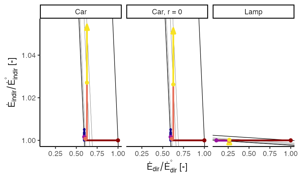
See help for path_graph_params for additional
information.
Sensitivity graphs
Sensitivity graphs can be created by the
sensitivity_graphs() function. A named list of sensitivity
parameters is required. These graphs are easiest described via
examples.
The first example shows the sensitivity of total rebound () to the macro parameter ().
df <- load_eeu_data()
sens_params <- list(Car = list(k = seq(0.5, 1.5, by = 0.5)),
                    Lamp = list(k = seq(0, 2, by = 1)))
sensitivity_graphs(rebound_data = df, parameterization = sens_params,
                   x_var = "k", y_var = "Re_tot") +
  ggplot2::facet_wrap(facets = "Case", scales = "free_x") +
  ggplot2::scale_colour_manual(values = c(Re_tot = "black"), guide = "none") +
  ggplot2::scale_discrete_manual(aesthetics = "linewidth", values = c(Re_tot = 0.5), guide = "none") +
  ggplot2::scale_linetype_manual(values = c(Re_tot = "solid"), guide = "none") +
  ggplot2::labs(y = expression(Re[tot]),
                colour = ggplot2::element_blank(),
                size = ggplot2::element_blank(),
                linetype = ggplot2::element_blank()) +
  ggplot2::theme_classic()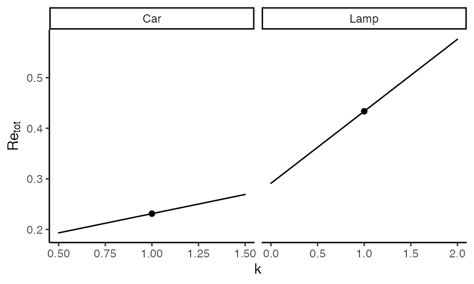
The next example shows multi-variate sensitivity. Values of the macro parameter () are shown in rows of the lattice plot. Uncompensated price elasticity of energy service consumption () is shown in columns of the lattice plot. Total rebound () is given on the -axis, and energy intensity of the economy () is given on the -axis. The cases (Car and Lamp) are shown as different lines.
sens_params_2 <- list(Car = list(k = seq(0, 2, by = 0.5),
                                 I_E = seq(2, 5, by = 1),
                                 e_qs_ps_UC_orig = seq(-0.5, -0.1, by = 0.1)),
                      Lamp = list(k = seq(0, 2, by = 0.5),
                                  I_E = seq(2, 5, by = 1),
                                  e_qs_ps_UC_orig = seq(-0.5, -0.1, by = 0.1)))
# Choose which rebound variables to include and their order.
sensitivity_graphs(rebound_data = df, parameterization = sens_params_2,
                   x_var = "I_E",
                   y_var = "Re_tot",
                   line_var = "Case") +
  ggplot2::facet_grid(rows = ggplot2::vars(k),
                      cols = ggplot2::vars(e_qs_ps_UC_orig), scales = "free_y") +
  ggplot2::scale_colour_manual(values = c(Car = "black", Lamp = "red")) +
  ggplot2::scale_discrete_manual(aesthetics = "linewidth", values = c(Car = 0.5, Lamp = 1.0)) +
  ggplot2::scale_linetype_manual(values = c(Car = "solid", Lamp = "dashed")) +
  ggplot2::labs(colour = ggplot2::element_blank(),
                size = ggplot2::element_blank(),
                linetype = ggplot2::element_blank(),
                linewidth = ggplot2::element_blank()) +
  ggplot2::theme_classic()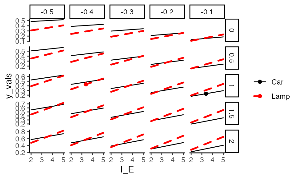
A third sensitivity example shows
sens_params_3 <- list(Car = list(eta_engr_units_star = seq(35, 50, by = 0.5)),
                      Lamp = list(eta_engr_units_star = seq(70, 90, by = 5)))
# Choose rebound terms to include in the graph and their order
rebound_vars <- c("Re_dempl", "Re_emb", "Re_omd", "Re_dsub", "Re_isub",
                  "Re_dinc", "Re_iinc", "Re_macro")

sensitivity_graphs(rebound_data = df, parameterization = sens_params_3,
                   x_var = "eta_engr_units_tilde",
                   y_var = rebound_vars) +
  ggplot2::facet_wrap(facets = "Case", scales = "free_x") +
  ggplot2::scale_colour_manual(values =
                                 c(Re_dempl = ReboundTools::path_graph_params$dempl_colour,
                                   Re_emb = ReboundTools::path_graph_params$emb_colour,
                                   Re_omd = ReboundTools::path_graph_params$md_colour,
                                   Re_dsub = ReboundTools::path_graph_params$dsub_colour,
                                   Re_isub = ReboundTools::path_graph_params$isub_colour,
                                   Re_dinc = ReboundTools::path_graph_params$dinc_colour,
                                   Re_iinc = ReboundTools::path_graph_params$iinc_colour,
                                   Re_macro = ReboundTools::path_graph_params$macro_colour),
                               breaks = rebound_vars) +
  ggplot2::scale_discrete_manual(aesthetics = "linewidth",
                                 values =
                                   c(Re_dempl = 0.2,
                                     Re_emb = ReboundTools::path_graph_params$emb_linewidth,
                                     Re_omd = ReboundTools::path_graph_params$md_linewidth,
                                     Re_dsub = ReboundTools::path_graph_params$dsub_linewidth,
                                     Re_isub = ReboundTools::path_graph_params$isub_linewidth,
                                     Re_dinc = ReboundTools::path_graph_params$dinc_linewidth,
                                     Re_iinc = ReboundTools::path_graph_params$iinc_linewidth,
                                     Re_macro = ReboundTools::path_graph_params$macro_linewidth),
                                 breaks = rebound_vars) +
  ggplot2::scale_linetype_manual(values =
                                   c(Re_dempl = ReboundTools::path_graph_params$dempl_linetype,
                                     Re_emb = ReboundTools::path_graph_params$emb_linetype,
                                     Re_omd = ReboundTools::path_graph_params$md_linetype,
                                     Re_dsub = ReboundTools::path_graph_params$dsub_linetype,
                                     Re_isub = "11",
                                     Re_dinc = ReboundTools::path_graph_params$dinc_linetype,
                                     Re_iinc = "11",
                                     Re_macro = ReboundTools::path_graph_params$macro_linetype),
                                 breaks = rebound_vars) +
  ggplot2::labs(x = expression(tilde(eta)*" [mpg (Car) or lm/W (Lamp)]"),
                y = "Re terms [-]",
                colour = ggplot2::element_blank(),
                size = ggplot2::element_blank(),
                linewidth = ggplot2::element_blank(),
                linetype = ggplot2::element_blank()) +
  ggplot2::theme_classic()
#> Warning: Removed 38 rows containing missing values or values outside the scale range
#> (`geom_path()`).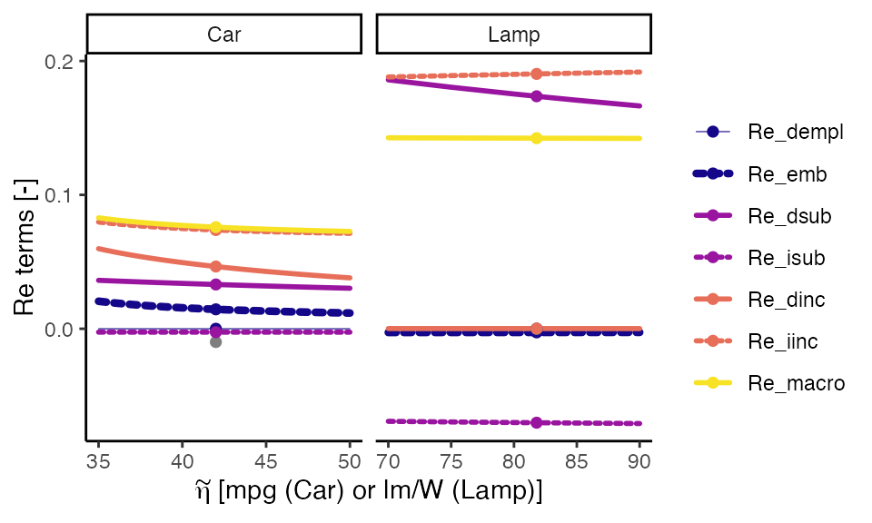
Conclusion
The ReboundTools package assists with analyzing rebound
effects and displaying the results. In particular,
- the
path_graphs()function returnsggplot2objects that show rebound path graphs and - the
sensitivity_graphs()function returnsggplot2objects that show sensitivity analyses.
Taken together, these functions provide important capabilities to analyze rebound effects for energy efficiency upgrades.