Using matsindf for principal components analysis
Alexander Davis
2025-11-18
Source:vignettes/iris_pca.Rmd
iris_pca.RmdIntroduction
When working with tidy data, it can be challenging to use R
operations that take in matrices. But the functions in
matsindf make it easier.
Data
We will illustrate how to handle these cases with
matsindf functions by doing principal components analysis
(PCA) on the classic Fisher iris dataset, often used to illustrate PCA.
We will be using a “long” input table, in which each measurement, rather
than each flower, is a single row.
long_iris <- datasets::iris %>%
  dplyr::mutate(flower = sprintf("flower_%d", 1:nrow(datasets::iris))) %>%
  tidyr::pivot_longer(
    cols = c(-Species, -flower), names_to = "dimension", values_to = "length"
  ) %>%
  dplyr::rename(species = Species) %>%
  dplyr::select(flower, species, dimension, length) %>%
  dplyr::mutate(species = as.character(species))

head(long_iris, n = 5)
#> # A tibble: 5 × 4
#>   flower   species dimension    length
#>   <chr>    <chr>   <chr>         <dbl>
#> 1 flower_1 setosa  Sepal.Length    5.1
#> 2 flower_1 setosa  Sepal.Width     3.5
#> 3 flower_1 setosa  Petal.Length    1.4
#> 4 flower_1 setosa  Petal.Width     0.2
#> 5 flower_2 setosa  Sepal.Length    4.9
Generate PCA results
Using matsindf, we can convert to a matrix, apply PCA,
and then convert back to a long format table.
long_pca_embeddings <- long_iris %>%
  collapse_to_matrices(
    rownames = "flower", colnames = "dimension", matvals = "length"
  ) %>%
  dplyr::transmute(projection = lapply(length, function(mat)
    stats::prcomp(mat, center = TRUE, scale = TRUE)$x
  )) %>%
  expand_to_tidy(
    rownames = "flower", colnames = "component", matvals = "projection"
  )
head(long_pca_embeddings, n = 5)
#>       flower component projection
#> 1   flower_1       PC1 -2.2571412
#> 2  flower_10       PC1 -2.1770349
#> 3 flower_100       PC1  0.2558734
#> 4 flower_101       PC1  1.8384100
#> 5 flower_102       PC1  1.1540156
The result are the coordinates of the iris data along the principal components, as a long format table. We just need to add back the species column …
long_pca_withspecies <- long_iris %>%
  dplyr::select(flower, species) %>%
  dplyr::distinct() %>%
  dplyr::left_join(long_pca_embeddings, by = "flower")
head(long_pca_withspecies, n = 5)
#> # A tibble: 5 × 4
#>   flower   species component projection
#>   <chr>    <chr>   <chr>          <dbl>
#> 1 flower_1 setosa  PC1          -2.26
#> 2 flower_1 setosa  PC2          -0.478
#> 3 flower_1 setosa  PC3           0.127
#> 4 flower_1 setosa  PC4          -0.0241
#> 5 flower_2 setosa  PC1          -2.07
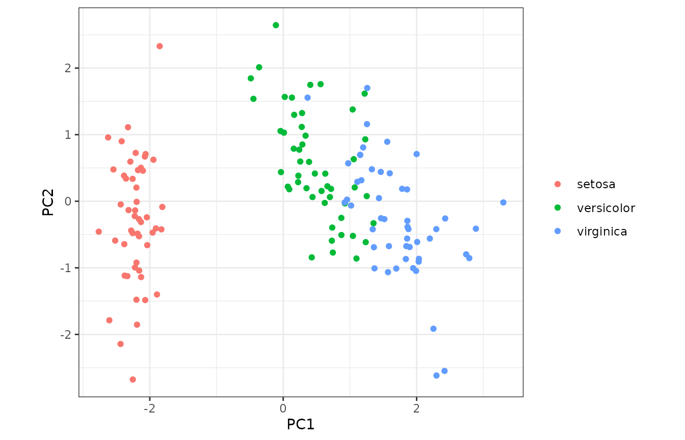
… followed by the familiar PCA plot.
long_pca_withspecies %>%
  tidyr::pivot_wider(
    id_cols = c(flower, species), names_from = component,
    values_from = projection
  ) %>%
  ggplot2::ggplot(ggplot2::aes(x = PC1, y = PC2, colour = species)) +
  ggplot2::geom_point() +
  ggplot2::labs(colour = ggplot2::element_blank()) +
  ggplot2::theme_bw() +
  ggplot2::coord_equal()
#> Warning: `label` cannot be a <ggplot2::element_blank> object.
As expected, we see that the distribution of measurements differs across the three species of iris.