Use Cases and Examples for matsindf

Introduction

Matrices are important mathematical objects, and they often describe networks of flows among nodes. Example networks are given in the following table.

System type	Flows	Nodes
Ecological	nutrients	organisms
Manufacturing	materials	factories
Economic	money	economic sectors

The power of matrices lies in their ability to organize network-wide calculations, thereby simplifying the work of analysts who study entire systems.

But wouldn’t it be nice if there were an easy way to create R data frames whose entries were not numbers but entire matrices? If that were possible, matrix algebra could be performed on columns of similar matrices.

That’s the reason for matsindf. It provides functions to convert a suitably-formatted tidy data frame into a data frame containing a column of matrices.

Furthermore, matsbyname is a sister package that

provides matrix algebra functions that respect names of matrix rows and columns (dimnames in R) to free the analyst from the task of aligning rows and columns of operands (matrices) passed to matrix algebra functions and
allows matrix algebra to be conducted within data frames using dplyr, tidyr, and other tidyverse functions.

When used together, matsindf and matsbyname allow analysts to wield simultaneously the power of both matrix mathematics and tidyverse functional programming.

This vignette demonstrates the use of these packages and suggests a workflow to accomplish sophisticated analyses using matrices in data frames (matsindf).

Data: `UKEnergy2000`

To demonstrate the use of matsindf functions, consider a network of energy flows from the environment, through transformation and distribution processes, and, ultimately, to final demand. Such energy flow networks are called energy conversion chains (ECCs), and this example is based on an approximation to a portion of the UK’s ECC circa 2000. (Note that these data are to be used for demonstration purposes only and have been rounded to 1–2 significant digits.) These example data first appeared in Figures 3 and 4 of Heun, Owen, and Brockway (2018).

head(UKEnergy2000, 2)
#>   Country Year Ledger.side      Flow.aggregation.point              Flow
#> 1      GB 2000      Supply Total primary energy supply Resources - Crude
#> 2      GB 2000      Supply Total primary energy supply    Resources - NG
#>   Product E.ktoe
#> 1   Crude  50000
#> 2      NG  43000

Country and Year contain only one value each, GB and 2000 respectively. Following conventions of the International Energy Agency’s energy balance tables,

Ledger.side indicates Supply or Consumption;
Flow.aggregation.point indicates how data are to be aggregated;
Flow indicates the industry, machine, or final demand sector for this flow;
Product indicates the energy carrier for this flow; and
E.ktoe gives the magnitude of this flow in units of kilotons of oil equivalent (ktoe).

Each flow is its own observation (its own row) in the UKEnergy2000 data frame, making it tidy.

The remainder of this vignette demonstrates an analysis conducted using the UKEnergy2000 data frame as a basis. It:

shows how to collapse and spread the data into appropriate matrices stored in columns of a data frame,
demonstrates analyzing the matrices with matsbyname functions,
illustrates expanding the matrices back into a tidy data frame, and
uses ggplot to graph the results.

Suggested workflow

Prepare for collapse

The EnergyUK2000 data frame is similar to “cleaned” data from an external source: there are no missing entries, and it is tidy. But the data are not organized as matrices, and additional metadata is needed.

The collapse_to_matrices function converts a tidy data frame into a matsindf data frame using using information within the tidy data frame. So the first task is to prepare for collapse by adding metadata columns.

collapse_to_matrices needs the following information:

argument to `collapse_to_matrices`	identifies
`matnames`	Name of the input column of matrix names
`values`	Name of the input column of matrix entries
`rownames`	Name of the input column of matrix row names
`colnames`	Name of the input column of matrix column name
`rowtypes`	Optional name of the input column of matrix row types
`coltypes`	Optional name of the input column of matrix column types

The following code gives the approach to adding metadata, appropriate for this application, relying on Ledger.side, the sign of E.ktoe, and knowledge about the rows and columns for each matrix. Each type of network will have its own algorithm for identifying row names, column names, row types, and column types in a tidy data frame.

UKEnergy2000_with_metadata <- UKEnergy2000 %>% 
  # Add a column indicating the matrix in which this entry belongs (U, V, or Y).
  matsindf:::add_UKEnergy2000_matnames() %>% 
  # Add columns for row names, column names, row types, and column types.
  matsindf:::add_UKEnergy2000_row_col_meta() %>% 
  mutate(
    # Eliminate columns we no longer need
    Ledger.side = NULL,
    Flow.aggregation.point = NULL,
    Flow = NULL,
    Product = NULL, 
    # Ensure that all energy values are positive, as required for analysis.
    E.ktoe = abs(E.ktoe)
  )
head(UKEnergy2000_with_metadata, 2)
#>   Country Year E.ktoe matname           rowname colname  rowtype coltype
#> 1      GB 2000  50000       V Resources - Crude   Crude Industry Product
#> 2      GB 2000  43000       V    Resources - NG      NG Industry Product

Collapse

With the metadata now in place, UKEnergy2000_with_metadata can be collapsed to a matsindf data frame by the collapse_to_matrices function. Much like dplyr::summarise, collapse_to_matrices relies on grouping to indicate which rows of the tidy data frame belong to which matrices. The usual approach is to tidyr::group_by the matnames column and any other columns to be preserved in the output, in this case Country and Year.

EnergyMats_2000 <- UKEnergy2000_with_metadata %>% 
  group_by(Country, Year, matname) %>% 
  collapse_to_matrices(matnames = "matname", matvals = "E.ktoe",
                       rownames = "rowname", colnames = "colname", 
                       rowtypes = "rowtype", coltypes = "coltype") %>% 
  rename(matrix.name = matname, matrix = E.ktoe)

# The remaining columns are Country, Year, matrix.name, and matrix
glimpse(EnergyMats_2000)
#> Rows: 3
#> Columns: 4
#> $ Country     <chr> "GB", "GB", "GB"
#> $ Year        <int> 2000, 2000, 2000
#> $ matrix.name <chr> "U", "V", "Y"
#> $ matrix      <list> <<matrix[11 x 9]>>, <<matrix[11 x 12]>>, <<matrix[4 x 2]>>

# To access one of the matrices, try one of these approaches:
(EnergyMats_2000 %>% filter(matrix.name == "U"))[["matrix"]] # The U matrix
#> [[1]]
#>                Oil fields Oil refineries Crude dist. Diesel dist.
#> Crude               50000              0           0            0
#> Crude - Dist.           0          47000           0            0
#> Crude - Fields          0              0       47500            0
#> Diesel                  0              0           0        15500
#> Diesel - Dist.         50              0          25            0
#> Elect                   0              0           0            0
#> Elect - Grid           25             75          25            0
#> NG                      0              0           0            0
#> NG - Dist.              0              0           0            0
#> NG - Wells              0              0           0            0
#> Petrol                  0              0           0            0
#>                Gas wells & proc. NG dist. Petrol dist. Elect. grid Power plants
#> Crude                          0        0            0           0            0
#> Crude - Dist.                  0        0            0           0            0
#> Crude - Fields                 0        0            0           0            0
#> Diesel                         0        0            0           0            0
#> Diesel - Dist.                50       25          250           0            0
#> Elect                          0        0            0        6400            0
#> Elect - Grid                  25       25            0           0          100
#> NG                         43000        0            0           0            0
#> NG - Dist.                     0        0            0           0        16000
#> NG - Wells                     0    41000            0           0            0
#> Petrol                         0        0        26500           0            0
#> attr(,"rowtype")
#> [1] "Product"
#> attr(,"coltype")
#> [1] "Industry"

EnergyMats_2000$matrix[[2]] # The V matrix
#>                   Crude - Dist. Diesel - Dist. Elect - Grid NG - Wells
#> Crude dist.               47000              0            0          0
#> Diesel dist.                  0          15150            0          0
#> Elect. grid                   0              0         6275          0
#> Gas wells & proc.             0              0            0      41000
#> NG dist.                      0              0            0          0
#> Oil fields                    0              0            0          0
#> Oil refineries                0              0            0          0
#> Petrol dist.                  0              0            0          0
#> Power plants                  0              0            0          0
#> Resources - Crude             0              0            0          0
#> Resources - NG                0              0            0          0
#>                   NG - Dist. Crude - Fields Diesel Petrol Petrol - Dist. Elect
#> Crude dist.                0              0      0      0              0     0
#> Diesel dist.               0              0      0      0              0     0
#> Elect. grid                0              0      0      0              0     0
#> Gas wells & proc.          0              0      0      0              0     0
#> NG dist.               41000              0      0      0              0     0
#> Oil fields                 0          47500      0      0              0     0
#> Oil refineries             0              0  15500  26500              0     0
#> Petrol dist.               0              0      0      0          26000     0
#> Power plants               0              0      0      0              0  6400
#> Resources - Crude          0              0      0      0              0     0
#> Resources - NG             0              0      0      0              0     0
#>                   Crude    NG
#> Crude dist.           0     0
#> Diesel dist.          0     0
#> Elect. grid           0     0
#> Gas wells & proc.     0     0
#> NG dist.              0     0
#> Oil fields            0     0
#> Oil refineries        0     0
#> Petrol dist.          0     0
#> Power plants          0     0
#> Resources - Crude 50000     0
#> Resources - NG        0 43000
#> attr(,"rowtype")
#> [1] "Industry"
#> attr(,"coltype")
#> [1] "Product"

EnergyMats_2000$matrix[[3]] # The Y matrix
#>                Transport Residential
#> Diesel - Dist.     14750           0
#> Elect - Grid           0        6000
#> NG - Dist.             0       25000
#> Petrol - Dist.     26000           0
#> attr(,"rowtype")
#> [1] "Product"
#> attr(,"coltype")
#> [1] "Sector"

Duplicate (for purposes of illustration)

Larger studies will include data for multiple countries and years. The ECC data from UK in year 2000 can be duplicated for 2001 and for a fictitious country AB. Although the data are unchanged, the additional rows serve to illustrate the functional programming aspects of the matsindf and matsbyname packages.

Energy <- EnergyMats_2000 %>% 
  # Create rows for a fictitious country "AB".
  # Although the rows for "AB" are same as the "GB" rows,
  # they serve to illustrate functional programming with matsindf.
  rbind(EnergyMats_2000 %>% mutate(Country = "AB")) %>% 
  spread(key = Year, value = matrix) %>% 
  mutate(
    # Create a column for a second year (2001).
    `2001` = `2000`
  ) %>% 
  gather(key = Year, value = matrix, `2000`, `2001`) %>% 
  # Now spread to put each matrix in a column.
  spread(key = matrix.name, value = matrix)

glimpse(Energy)
#> Rows: 4
#> Columns: 5
#> $ Country <chr> "AB", "AB", "GB", "GB"
#> $ Year    <chr> "2000", "2001", "2000", "2001"
#> $ U       <list> <<matrix[11 x 9]>>, <<matrix[11 x 9]>>, <<matrix[11 x 9]>>, <<…
#> $ V       <list> <<matrix[11 x 12]>>, <<matrix[11 x 12]>>, <<matrix[11 x 12]>>,…
#> $ Y       <list> <<matrix[4 x 2]>>, <<matrix[4 x 2]>>, <<matrix[4 x 2]>>, <<ma…

Verify data

An important step in any analysis is data verification. For an ECC analysis, it is important to verify that energy is conserved (i.e., energy is in balance) across all industries. Equations 1 and 2 in Heun, Owen, and Brockway (2018) show that energy balance is verified by

$\mathbf{W} = \mathbf{V}^\mathrm{T} - \mathbf{U},$

and

$\mathbf{W}\mathbf{i} - \mathbf{Y}\mathbf{i} = \mathbf{0}.$

Energy balance verification can be implemented with matsbyname functions and tidyverse functional programming:

Check <- Energy %>% 
  mutate(
    W = difference_byname(transpose_byname(V), U),
    # Need to change column name and type on y so it can be subtracted from row sums of W
    err = difference_byname(rowsums_byname(W), 
                            rowsums_byname(Y) %>% 
                              setcolnames_byname("Industry") %>% setcoltype("Industry")),
    EBalOK = iszero_byname(err)
  )
Check %>% select(Country, Year, EBalOK)
#>   Country Year EBalOK
#> 1      AB 2000   TRUE
#> 2      AB 2001   TRUE
#> 3      GB 2000   TRUE
#> 4      GB 2001   TRUE
all(Check$EBalOK %>% as.logical())
#> [1] TRUE

This example demonstrates that energy balance can be verified for all combinations of Country and Year with a few lines of code. In fact, the exact same code can be applied to the Energy data frame, regardless of the number of rows in it.

Secure in the knowledge that energy is conserved across all ECCs in the Energy data frame, other analyses can proceed.

Efficiencies

To further illustrate the power of matsbyname functions in the context of matsindf, consider the calculation of the efficiency of every industry in the ECC as column vector $\eta$ as shown by Equation 11 of Heun, Owen, and Brockway (2018).

$\mathbf{g} = \mathbf{V}\mathbf{i}$

$\mathbf{\eta} = \widehat{\mathbf{U}^\mathrm{T} \mathbf{i}}^{\mathrm{-}1} \mathbf{g}$

Etas <- Energy %>% 
  mutate(
    g = rowsums_byname(V),
    eta = transpose_byname(U) %>% rowsums_byname() %>% 
      hatize_byname(keep = "rownames") %>% invert_byname() %>% 
      matrixproduct_byname(g) %>% 
      setcolnames_byname("eta") %>% setcoltype("Efficiency")
  ) %>% 
  select(Country, Year, eta)

Etas$eta[[1]]
#>                         eta
#> Crude dist.       0.9884332
#> Diesel dist.      0.9774194
#> Elect. grid       0.9804688
#> Gas wells & proc. 0.9518282
#> NG dist.          0.9987820
#> Oil fields        0.9485771
#> Oil refineries    0.8921933
#> Petrol dist.      0.9719626
#> Power plants      0.3975155
#> attr(,"rowtype")
#> [1] "Industry"
#> attr(,"coltype")
#> [1] "Efficiency"

Note that only a few lines of code are required to perform the same series of matrix operations on every combination of Country and Year. In fact, the same code will be used to calculate the efficiency of any number of industries in any number of countries and years!

Expand

Plotting values from a matsindf data frame can be accomplished by expanding the matrices of the matsindf data frame (in this example, Etas) back out to a tidy data frame. Expanding is the reverse of collapse-ing, and the following information must be supplied to the expand_to_tidy function:

argument to `expand_to_tidy`	identifies
`matnames`	Name of the input column of matrix names
`matvals`	Name of the input column of matrices to be expanded
`rownames`	Name of the output column of matrix row names
`colnames`	Name of the output column of matrix column name
`rowtypes`	Optional name of the output column of matrix row types
`coltypes`	Optional name of the output column of matrix column types
`drop`	Optional value to be dropped from output (often 0)

Prior to expanding, it is usually necessary to gather columns of matrices.

etas_forgraphing <- Etas %>% 
  gather(key = matrix.names, value = matrix, eta) %>% 
  expand_to_tidy(matnames = "matrix.names", matvals = "matrix", 
                 rownames = "Industry", colnames = "etas", 
                 rowtypes = "rowtype", coltypes = "Efficiencies") %>% 
  mutate(
    # Eliminate columns we no longer need.
    matrix.names = NULL,
    etas = NULL, 
    rowtype = NULL, 
    Efficiencies = NULL
  ) %>% 
  rename(
    eta = matrix
  )

# Compare to Figure 8 of Heun, Owen, and Brockway (2018)
etas_forgraphing %>% filter(Country == "GB", Year == 2000)
#> # A tibble: 9 × 4
#>   Country Year  Industry            eta
#>   <chr>   <chr> <chr>             <dbl>
#> 1 GB      2000  Crude dist.       0.988
#> 2 GB      2000  Diesel dist.      0.977
#> 3 GB      2000  Elect. grid       0.980
#> 4 GB      2000  Gas wells & proc. 0.952
#> 5 GB      2000  NG dist.          0.999
#> 6 GB      2000  Oil fields        0.949
#> 7 GB      2000  Oil refineries    0.892
#> 8 GB      2000  Petrol dist.      0.972
#> 9 GB      2000  Power plants      0.398

etas_forgraphing is a data frame of efficiencies, one for each Country, Year, and Industry, in a format that is amenable to plotting with packages such as ggplot.

Report

The following code creates a bar graph of efficiency results for the UK in 2000:

etas_UK_2000 <- etas_forgraphing %>% filter(Country == "GB", Year == 2000) 

etas_UK_2000 %>% 
  ggplot(mapping = aes_string(x = "Industry", y = "eta", 
                              fill = "Industry", colour = "Industry")) + 
  geom_bar(stat = "identity") +
  labs(x = NULL, y = expression(eta[UK*","*2000]), fill = NULL) + 
  scale_y_continuous(breaks = seq(0, 1, by = 0.2)) +
  scale_fill_manual(values = rep("white", nrow(etas_UK_2000))) +
  scale_colour_manual(values = rep("gray20", nrow(etas_UK_2000))) + 
  guides(fill = FALSE, colour = FALSE) +
  theme(axis.text.x = element_text(angle = 90, vjust = 0.4, hjust = 1))
#> Warning: `aes_string()` was deprecated in ggplot2 3.0.0.
#> ℹ Please use tidy evaluation idioms with `aes()`.
#> ℹ See also `vignette("ggplot2-in-packages")` for more information.
#> This warning is displayed once every 8 hours.
#> Call `lifecycle::last_lifecycle_warnings()` to see where this warning was
#> generated.
#> Warning: The `<scale>` argument of `guides()` cannot be `FALSE`. Use "none" instead as
#> of ggplot2 3.3.4.
#> This warning is displayed once every 8 hours.
#> Call `lifecycle::last_lifecycle_warnings()` to see where this warning was
#> generated.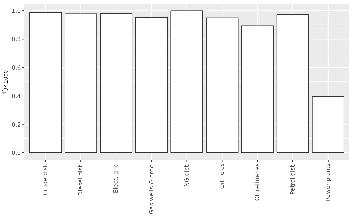

Conclusion

This vignette demonstrated the use of the matsindf and matsbyname packages and suggested a workflow to accomplish sophisticated analyses using matrices in data frames (matsindf).

The workflow is as follows:

Reshape data into a tidy data frame with columns for matrix name, element value, row name, column name, row type, and column type, similar to UKEnergy2000 above.
Use collapse_to_matrices to create a data frame of matrices with columns for matrix names and matrices themselves, similar to EnergyMats_2000 above.
tidyr::spread the matrices to obtain a data frame with columns for each matrix, similar to Energy above.
Validate the data, similar to Check above.
Perform matrix algebra operations on the columns of matrices using matsbyname functions in a manner similar to the process of generating the Etas data frame above.
tidyr::gather the columns to obtain a tidy data frame of matrices.
Use expand_to_tidy to create a tidy data frame of matrix elements, similar to etas_forgraphing above.
Plot and report results as demonstrated by the graph above.

Data frames of matrices, such as those created by matsindf, are like magic spreadsheets in which single cells contain entire matrices. With this data structure, analysts can wield simultaneously the power of both matrix mathematics and tidyverse functional programming.

References

Heun, Matthew Kuperus, Anne Owen, and Paul E. Brockway. 2018. “A Physical Supply-Use Table Framework for Energy Analysis on the Energy Conversion Chain.” Applied Energy 226 (September): 1134–62. https://doi.org/10.1016/j.apenergy.2018.05.109.

Matthew Kuperus Heun

2025-05-26

Introduction

Data: `UKEnergy2000`

Suggested workflow

Prepare for collapse

Collapse

Duplicate (for purposes of illustration)

Verify data

Efficiencies

Expand

Report

Conclusion

References

Use Cases and Examples for matsindf

Matthew Kuperus Heun

2025-05-26

Introduction

Data: UKEnergy2000

Suggested workflow

Prepare for collapse

Collapse

Duplicate (for purposes of illustration)

Verify data

Efficiencies

Expand

Report

Conclusion

References

Data: `UKEnergy2000`